A production manager rarely asks, “What's the payback period?” in isolation. The question is harder: should we retrofit the existing station, add semi-automatic assistance, or commit to a fully automated line? Each option changes labor exposure, throughput, quality risk, flexibility, commissioning effort, and the amount of capital tied up before the plant sees a return.
That's why learning how to calculate payback period matters for more than finance approval. Used properly, it turns a messy manufacturing decision into a recovery timeline you can challenge, compare, and defend. Used carelessly, it rewards optimistic vendor assumptions and makes an expensive project look safer than it is.
Table of Contents
- The Decision Operations Managers Actually Face
- The Simple Payback Formula with Two Worked Examples
- Discounted Payback and Why It Changes the Answer
- Benchmark Ranges for Automation Projects
- Building the Calculation in Excel
- Reading the Result with Eyes Open
- A Practical Checklist Before You Sign Off
The Decision Operations Managers Actually Face
Lena is standing beside a two-shift assembly line at a Tier-1 automotive supplier, reviewing a quote for a $180,000 semi-automatic assembly cell. The line uses four operators per shift. Scrap is running at 3.2%, and an ergonomics claim may force the plant to redesign the workstation whether the capital project proceeds or not.
Her alternatives are concrete. She can purchase the semi-automatic cell, retrofit one station for roughly $65,000, or continue operating as-is while labor and quality costs rise. The finance team wants one number. The operations team knows that the number depends on what gets counted.
A credible payback model starts with the total installed investment, not the equipment price on the quotation. Installation, tooling, controls integration, training, commissioning, software, spares, and ramp-up labor belong in the cost base. Guidance for automation projects specifically recommends using fully loaded cash flows and including maintenance, spares, software, integration, training, commissioning, and lost flexibility where those costs are traceable. Automation payback guidance for engineering projects
What belongs in the recovery calculation
Lena should quantify benefits that the plant can verify:
- Labor hours released: Use time studies and the actual staffing plan, not theoretical headcount elimination.
- Scrap reduction: Use quality records to establish the current loss and model only the improvement the process can support.
- Cycle-time improvement: Count throughput only when demand, downstream capacity, and actual run time support the additional output.
- Avoided injury cost: Include documented claims, modified-duty exposure, and engineering actions that the project removes.
- Ongoing operating cost: Subtract maintenance, consumables, software, utilities, and support requirements from annual benefits.
The figures that often make a model look better without creating cash are different. Allocated corporate overhead doesn't automatically disappear when a cell is installed. Theoretical capacity isn't a throughput gain unless the plant can sell, schedule, and support the output. A labor “saving” isn't real if the operators move to another bottleneck.
Practical rule: If nobody can point to the payroll record, quality report, maintenance log, production schedule, or approved cost estimate behind an input, label it an assumption.
The payback period is useful because it compresses that debate into one question: when does cumulative net cash flow recover the upfront investment? It doesn't decide which automation level is strategically right, but it gives Lena a defensible screening figure for her VP of Operations.
The Simple Payback Formula with Two Worked Examples
For even cash flows, the formula is direct:
Payback Period = Initial Investment ÷ Average Annual Net Cash Inflow
The phrase net cash inflow matters. It means the annual benefit after ongoing project costs, not gross savings or revenue that hasn't been realized. The payback method became widely used because it answers a simple operational question quickly and can be applied without an elaborate financial model. Overview of the payback method
Example A with even annual savings
A cobot cell requires $150,000 and produces $50,000 per year in net savings.
$150,000 ÷ $50,000 = 3.0 years
The cumulative calculation confirms the result:
| Year | Net Cash Flow ($) | Cumulative Cash Flow ($) |
|---|---|---|
| 0 | -150,000 | -150,000 |
| 1 | 50,000 | -100,000 |
| 2 | 50,000 | -50,000 |
| 3 | 50,000 | 0 |
This is the situation where simple division works. The annual cash inflow is stable, and the project recovers at the end of year three.
Example B with an uneven ramp
Now consider a $250,000 semi-automatic line. The project generates $40,000 in year one, $80,000 in year two, and $95,000 in years three through five. The first year is weaker because operators are learning the process and the line is still being tuned.
| Year | Investment ($) | Net Cash Flow ($) | Cumulative Cash Flow ($) | Notes |
|---|---|---|---|---|
| 0 | -250,000 | 0 | -250,000 | Initial installed investment |
| 1 | 0 | 40,000 | -210,000 | Ramp-up year |
| 2 | 0 | 80,000 | -130,000 | Stabilizing output |
| 3 | 0 | 95,000 | -35,000 | Recovery not yet reached |
| 4 | 0 | 95,000 | 60,000 | Recovery occurs during year four |
| 5 | 0 | 95,000 | 155,000 | Cash after recovery |
At the end of year three, $35,000 remains unrecovered. Divide that balance by the year-four inflow:
$35,000 ÷ $95,000 = 0.37
The simple payback is therefore approximately 3.4 years, based on these stated cash flows. The arithmetic must follow the table. If a model shows 3.6 years, check whether its year-four cash flow or cost treatment differs from the figures entered.
The most common errors occur before the formula is applied. Teams forget residual capital spending buried in year-one installation, or they omit salvage value entirely instead of placing it in the appropriate cash-flow period. For uneven returns, use cumulative net cash flow and interpolate within the recovery year, as described in investment appraisal guidance for uneven cash flows. A practical labor-cost model can also help separate genuine labor reduction from hours merely reassigned to another task, using this labor cost reduction framework.
Discounted Payback and Why It Changes the Answer
Simple payback treats a dollar received sooner the same as a dollar received later. That weakness matters when a project takes several years to recover, when the cost of capital is high, or when a plant must choose between competing uses for limited capital.
Discounted payback corrects for that timing. Each future cash flow is converted to present value using the firm's hurdle rate, then added cumulatively until the discounted total recovers the investment. The method preserves the intuitive recovery question while recognizing the time value of money. Explanation of discounted payback
Applying a 12% hurdle rate
For a cash flow received in year t, the present-value calculation is:
Discounted Cash Flow = Cash Flow ÷ (1 + r)^t
Here, r is the 12% discount rate and t is the year. Applying that rate to Example B gives the following values:
| Year | Net Cash Flow ($) | Discount Factor (12%) | Discounted Cash Flow ($) | Cumulative Discounted ($) |
|---|---|---|---|---|
| 0 | -250,000 | 1.0000 | -250,000 | -250,000 |
| 1 | 40,000 | 0.8929 | 35,714 | -214,286 |
| 2 | 80,000 | 0.7972 | 63,776 | -150,510 |
| 3 | 95,000 | 0.7115 | 67,597 | -82,913 |
| 4 | 95,000 | 0.6350 | 60,355 | -22,558 |
The displayed four-year cash flows still leave a negative cumulative discounted balance. Recovery would therefore occur later than year four if the project continues producing the stated annual benefit. A claim that this exact table produces a discounted payback of roughly 4.2 years doesn't reconcile mathematically with the listed figures. The correct engineering response is to flag the inconsistency, not force the spreadsheet to match the expected answer.
Finance discipline: The discount rate belongs in the model before the project is ranked, not after the preferred project has already been chosen.
Why project rankings can change
A retrofit may have a lower upfront cost and a faster simple recovery because it produces modest savings quickly. A larger automated line may require more capital but generate stronger later-year savings. Discounting reduces the present value of those later benefits, so the larger project can lose its apparent advantage even when its lifetime cash contribution is greater.
That is why the simple and discounted results should sit side by side. Neutral guidance describes payback as a recovery measure and discounted payback as recovery after applying a hurdle rate or WACC. Payback period and discounted payback comparison
A project that never recovers on a discounted basis within the analysis horizon isn't automatically worthless. It has failed the payback screen. Evaluate it with NPV, IRR, strategic necessity, risk, and asset life before rejecting it.
Benchmark Ranges for Automation Projects
Benchmarking helps identify a calculation that deserves scrutiny, but it doesn't replace plant-specific data. Scope, product mix, staffing, uptime, quality losses, and integration complexity can move the result substantially.
Industry guidance commonly places many well-scoped manufacturing automation deployments in the 12 to 24 month range, while complex custom or multi-system projects can extend into the 24 to 48 month range. Manufacturing automation investment guidance
Collaborative robots are often positioned at the faster-payback end, with cited ranges from 6 to 18 months, 8 to 18 months, or 8 to 14 months, depending on the application. Heavier six-axis industrial cells are commonly cited at about 14 to 24 months or longer. Robot ROI and payback comparisons
| Automation Level | Typical Investment | Payback Range | Main Driver |
|---|---|---|---|
| Cobot workstation | $40K to $90K | 6 to 14 months | Targeted labor and ergonomic improvement |
| Semi-automatic cell | $120K to $250K | 12 to 24 months | Balanced labor, quality, and throughput gains |
| Fully automated line | $500K to $2M+ | 30 to 60 months | High integration cost and larger later-stage capacity |
These investment and payback ranges are benchmark figures, not promises. The cited guidance describes cobot applications as faster-payback projects, while broader automation sources also report longer windows for custom deployments. Vendor brochures frequently show best-case utilization, ideal staffing assumptions, and uninterrupted demand.
Compare scope with scope
A semi-automatic cell shouldn't be judged against the payback claim for a small cobot workstation. A fully integrated line may include conveyors, vision, safety systems, material handling, software, validation, and plant interfaces that a workstation doesn't require.
A useful benchmark review asks:
- Does the scope match? Compare installed systems with installed systems.
- Does the benefit source match? Labor savings, scrap reduction, and throughput should be defined consistently.
- Does the operating context match? A high-volume product may support automation that a variable-mix line cannot.
One manufacturing automation guide describes under 12 months as a strong case, 18 to 24 months as defensible for high-value equipment, and anything beyond that as requiring a second look against baseline evidence. Automation ROI validation guidance
Building the Calculation in Excel
A workable spreadsheet should let operations, engineering, and finance inspect the same assumptions. Keep the layout visible. Hiding installation, training, or maintenance in a single “project cost” cell makes review difficult and encourages arguments about the answer instead of the inputs.
Start with one row per period and these columns:
| Column | Purpose |
|---|---|
| A | Year |
| B | Investment or net cash flow |
| C | Cumulative cash flow |
| D | Discounted cash flow |
| E | Cumulative discounted cash flow |
| F | Payback flag |
Use Year 0 for the initial outlay. Put operating cash inflows in Year 1 through Year 5, or extend the horizon for equipment with a longer useful life. Net each year's savings against maintenance, software, consumables, additional staffing, and other traceable operating costs.
Insert the required spreadsheet visual near the start of the model-building work:

Formulas that make the sheet auditable
If the annual rate is stored in cell H1, calculate present value in the Year 1 row with either:
=PV($H$1,A2,-B2)
or:
=-B2/(1+$H$1)^A2
Use the second form when you want the mechanics to remain obvious to reviewers. Copy it down for each operating year, then calculate cumulative discounted cash flow as a running total.
For a simple payback flag, the required conditional formula is:
=IF(C2<0,IF(C3>=0,B3+ABS(C2)/D3,"Not recovered"),"")
The formula assumes the row above contains the last negative cumulative value, the next row contains the recovery-period cash flow, and the column references match your layout. Test it against a known example before using it for an approval package.
Modeling habit: Add a notes column beside every assumption. Record whether the input came from a time study, maintenance history, quality report, labor rate, supplier quotation, or management estimate.
Apply conditional formatting to the cumulative column. Highlight cells at or above zero in green and negative cells in red. The recovery cell becomes immediately visible during a review, while an unrecovered project remains obvious rather than being buried in a summary page.
A two-variable data table adds more value than polishing the headline number. Put the discount rate on one axis and the annual savings variation on the other. The resulting grid shows how quickly payback shifts when finance changes the hurdle rate or operations changes the benefit assumption.
For a separate starting point, compare the completed model with an automation ROI calculator, then reconcile every difference. A calculator can accelerate screening, but your plant records should control the final case.
Use the video only after the spreadsheet structure and formulas are in place, so the visual walkthrough reinforces a model you understand:
Reading the Result with Eyes Open
A 14-month payback on a $200,000 cell isn't automatically better than a 28-month payback on a $1.2 million line. The larger line may generate cash for 12 years, while the smaller project may have limited output, greater manual dependence, or less value after its first application. Those figures are useful only when they sit beside the full cash-flow profile.
Four questions beyond the recovery date
Residual value matters when the equipment can be redeployed, sold, or adapted. Include a defensible terminal value in the model rather than treating the asset as worthless without investigation.
Flexibility can outweigh speed. A dedicated line locked to one product may recover quickly but leave the plant exposed when mix changes. A retrofit or semi-automatic station may preserve operator involvement and make future tooling changes easier.
Obsolescence creates a different risk. Technology that becomes difficult to support before the asset is paid off can produce a deceptively attractive early result. Review controls architecture, spare-part availability, software support, and the expected product roadmap.
Post-payback contribution is where long-life projects often earn their justification. Payback ignores cash flows after recovery, which means it can rank a short, thin project above a slower project with stronger lifetime value. Investment appraisal limitations
Plot cumulative cash flow through year 8 or year 10 when the project life supports it. The shape tells you whether the investment produces a durable operating advantage or merely clears the approval gate.
The uncomfortable test: If payback arrives close to the useful life of the technology, the project has little room for commissioning delays, downtime, demand loss, or redesign.
Total cost of ownership makes these trade-offs easier to see because it keeps acquisition, operation, support, and replacement considerations together. Use a total cost of ownership framework alongside payback rather than allowing the recovery date to stand alone.
A Practical Checklist Before You Sign Off
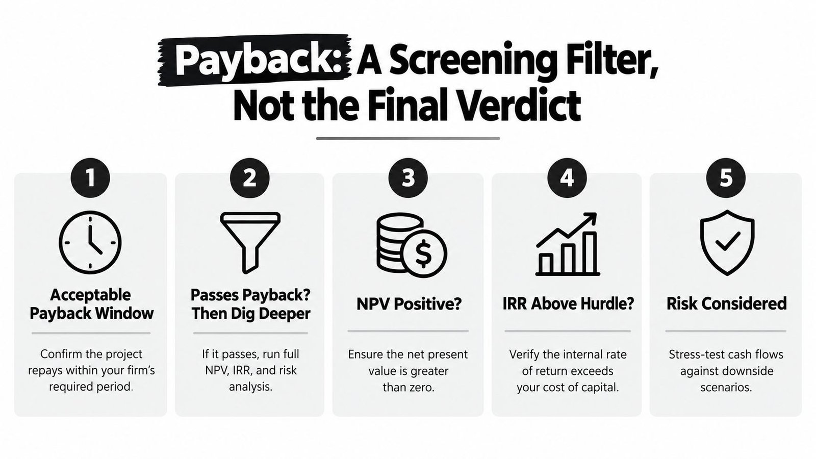
Treat payback as a screening filter, not the final verdict. It can eliminate a project that won't return capital within the company's acceptable window, but a project that passes still needs NPV, IRR, operational validation, and downside analysis.
Before signing off, run this factory review:
- Confirm the complete outlay. Include equipment, installation, tooling, training, commissioning, and a realistic contingency. A contingency of 10% to 15% is commonly used in the stated approval guidance, but finance and engineering should agree on the amount for the specific scope.
- Trace annual savings. Tie labor benefits to time studies, scrap benefits to quality reports, and labor rates to approved finance data.
- Separate revenue uplift. Pressure-test additional revenue independently from cost reduction. Don't use uncommitted demand to rescue a weak automation case.
- Check concentration risk. Identify dependence on one customer, SKU, shift pattern, or production schedule.
- Agree on the discount rate. Finance should approve the hurdle rate before engineering compares alternatives.
- Revisit major assumption changes. Re-run the model when commodity prices or volumes shift by more than 10%, as specified in the operating review checklist.
- Document downtime exposure. Record which savings stop immediately when the line is down and which benefits continue.
- Validate maintenance ownership. Assign responsibility for preventive maintenance, spare parts, controls support, and recovery after faults.
- Model the ramp. Include installation, onboarding, training, commissioning, and ramp-up hours before full benefits appear.
- Name the savings owner. One person should track actual labor, scrap, quality, throughput, and maintenance results after launch.
The operations leader who signs the approval will usually be asked later why actual savings lagged the model. A documented baseline, named owners, traceable inputs, and a clear recovery rule provide the defense. They also make it easier to correct the project while the equipment is still being commissioned.
The right decision isn't always the shortest payback. It's the automation level that returns capital within the firm's risk tolerance while preserving the quality, flexibility, safety, and production performance the plant needs.
System Engineering & Automation provides semi-automatic systems, fully automated and manual equipment, custom tooling, fixtures, integrated controls, installation, commissioning, and ongoing support for manufacturing operations. Visit System Engineering & Automation to discuss a payback model grounded in your actual process data and identify an automation solution that fits your production goals and budget.